Latent Thought Flows with Text Compression
Released on Jun 9th, 2026
For images, audio, video, and actions, modern generative modeling increasingly shares one recipe: compress the signal into continuous latent tokens, train a generator to map noise to those tokens, and decode them back into the original domain [13].
Language has been the exception.
Text is not raw sensory data. It is a human-made compression of perception, memory, intent, and world state into symbols. Tokenization compresses it again, but still leaves a long sequence of discrete units. This raises a central question:
Can text — discrete and compressed to begin with — be further compressed into a short sequence of continuous latents that is useful for generation?
This is not just an efficiency question. If text cannot be moved into a compact continuous latent space, unified latent generative modeling has a structural asymmetry: images, audio, video, and actions live in continuous latent spaces, while language remains a long stream of discrete symbols. If text can be represented similarly, language shares the same modeling interface as every other modality.
Our core message is simple: text can be compressed into a short sequence of continuous latents that remains useful for generation. This lets language share the same latent-generative recipe as the other modalities, while a text decoder handles surface realization.
Motivation
There are three reasons to care.
First, this is a missing piece for unified generative modeling. A system that represents images, audio, video, actions, and text in compatible continuous spaces is easier to compose than one where language must always be handled as an exceptional discrete stream.
Second, compression has always been central to intelligence [1]. A useful representation discards irrelevant detail while preserving what is needed for prediction and control. Language is already an extraordinary compression scheme — but perhaps not a complete one: a single thought still unfolds across many tokens. Another level of compression could help — a compact latent state for an entire span of text.
Third, compression can buy efficiency. Reducing the number of generated tokens is one of the most direct ways to reduce latency and long-context cost. Prior work on neural text, prompt, and context compression already shows that learned summary tokens can reduce repeated context processing [2, 14, 15]. We want to go further: a good latent text model should generate a short sequence of continuous tokens and then read it out into text, instead of making every semantic decision at the original token length.
Why Text Latents Are Hard
The difficulty is that text is already discrete, sparse, and highly compressed. A continuous autoencoder can easily learn to reconstruct text while producing a latent space with poor geometry. A strong decoder may ignore the latents; a weak bottleneck may destroy semantics; a reconstruction metric may look excellent even when interpolation collapses.
This is the main trap. If we only ask whether the readout decoder can recover the input text, we are testing a reconstruction system, not a generative representation.
There are two failure modes we need to avoid. The first is representation collapse: the autoencoder reconstructs well, but the latent codes do not organize into a smooth space for interpolation or generation. The second is latent underuse, often discussed as posterior collapse in language VAEs [5, 8, 12]: a strong readout decoder can achieve low reconstruction loss from local textual context and its language prior, without being forced to rely on the latent sequence. The issue is not that underuse improves reconstruction; it is that reconstruction loss may fail to reveal whether the latent was actually used. In both cases, reconstruction can look good while the learned latents remain poor generative objects.
The desired latent space should satisfy stronger properties:
- It should preserve global sequence information.
- It should support interpolation between examples.
- It should be easy for a continuous generator to model.
This motivates two choices. First, the training task should stress the bottleneck: the encoder should not be able to pass token-level details through unchanged, and the decoder should not be able to ignore the encoder's output. Second, evaluation should test latent geometry and generated distributions, not only reconstruction.
What Are Latent Thought Flows?

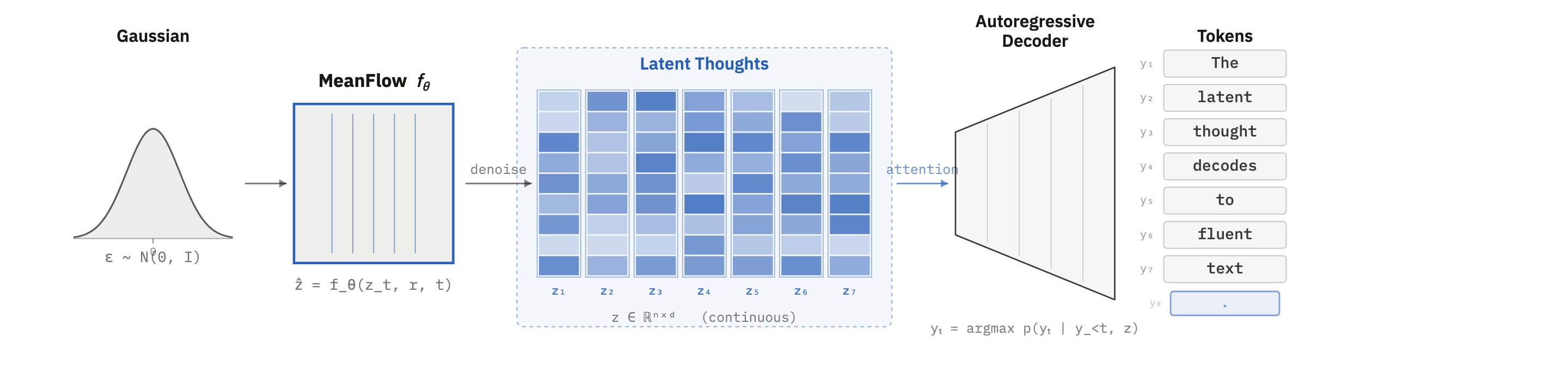
Latent Thought Flows generation. A MeanFlow model [24] maps Gaussian noise into a short sequence of continuous latent tokens in a single step, and the readout decoder expands them back into text.
Latent Thought Flows = text autoencoder + continuous latent generator + readout decoder. The autoencoder compresses a long token sequence into K continuous latent tokens; the latent generator samples those tokens directly; and the readout decoder maps them back into text. The current implementation uses an autoregressive readout, but the core component is the short continuous latent sequence, not the particular readout architecture.
The key point is that we are not diffusing text itself. We are modeling the low-dimensional manifold of valid text latents: the set of continuous latent sequences produced by the encoder that the readout decoder knows how to turn back into coherent text.
In our experiments, this means compressing a 256-token text patch into 8 continuous latent tokens.
Better Quality at the Same Inference Cost
Compressing text into a short latent sequence and then generating in that compressed space offers a direct efficiency dividend: the latent generator operates on K continuous tokens instead of L text tokens, with K \ll L. But the more immediate payoff in our current system is quality. In this TinyStories [25] setting, Latent Thought Flows produce higher-quality text than autoregressive generation at matched inference FLOPs.
Here gMAUVE is MAUVE [7] computed between generated samples and held-out real text; higher is better, with 1.0 indicating a closer match to the reference distribution. We define the full metric family below.
The result can be summarized in three lines:
- LTF beats token AR at matched inference cost.
- The latent-flow overhead is small in this compressed setting.
- Diversity comes from the latent generator, not decoder temperature.
Same readout scale, better generation
The first comparison asks whether conditioning a readout decoder on a latent prefix from the flow model improves generation quality over running an autoregressive model directly over tokens. We use the same TinyStories setting and sweep the same decoder/readout scales. The AR baseline is independently tuned over learning rate, weight decay, and sampling temperature. LTF uses a 5M-parameter MeanFlow model with one-step sampling, and the x-axis includes the extra flow cost.
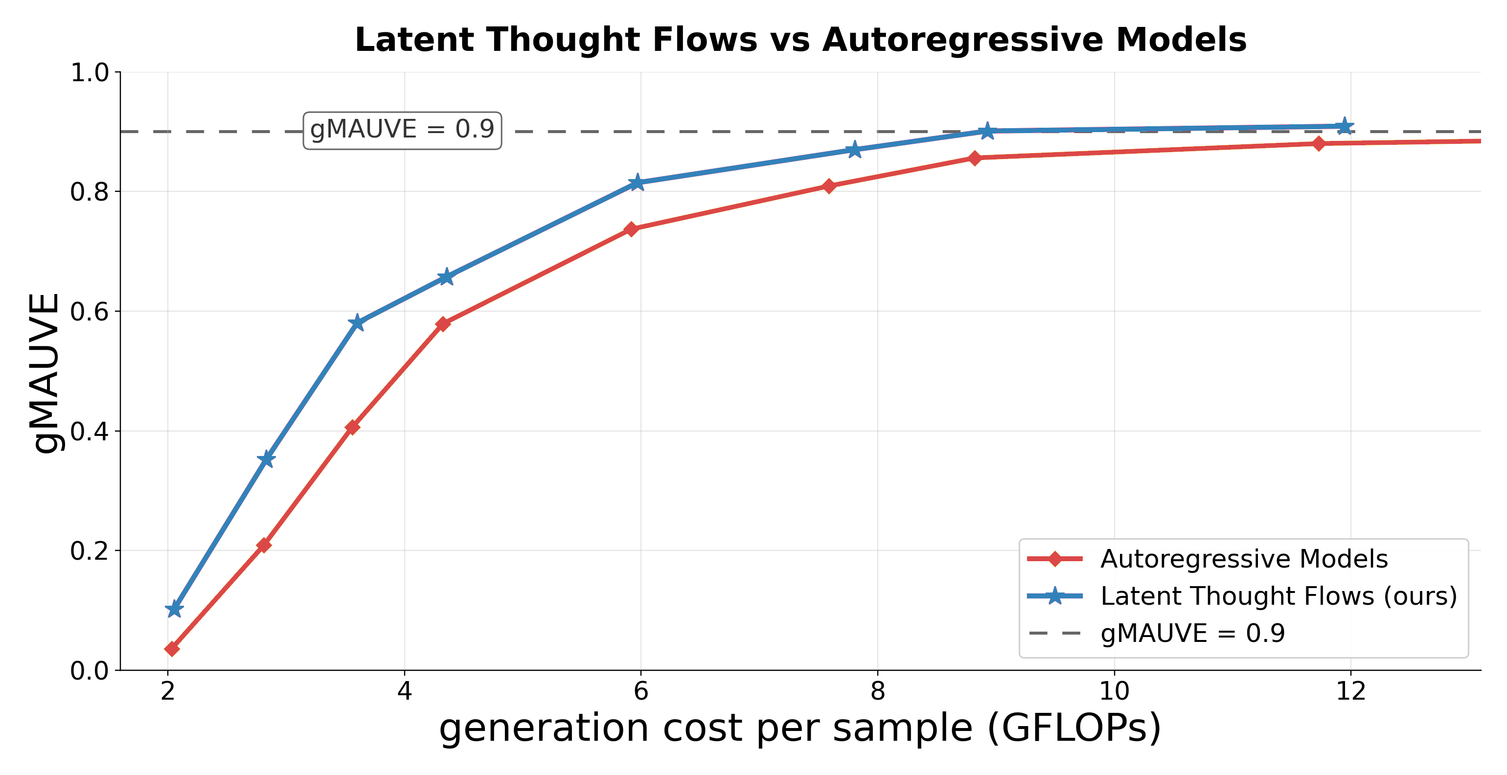
TinyStories quality-compute frontier. Latent Thought Flows (blue) stay above the independently tuned token-AR baseline (red) across the shared cost range and cross gMAUVE 0.9.
The flow model adds a small inference cost
The result above is notable because the latent generator is compact: in this TinyStories K=8 setting, a 5M-parameter one-step MeanFlow model is enough to shift the readout decoder onto a better quality-compute frontier. One might worry that adding this flow model on top of the decoder creates a significant inference overhead. Compression is what keeps this cost acceptable: the flow model operates on K latent tokens rather than L text tokens, and we use MeanFlow, which generates in a single step. Using the standard dense-Transformer FLOPs proxy from language-model scaling estimates [22, 23], the flow model cost is approximately one forward pass over K latent tokens:
For our compact flow model (N_{\text{flow}} \approx 5\text{M}, K = 8 latent tokens), this is about 80 MFLOPs per sample — compared to 2–9 GFLOPs for the decoder alone. The flow model adds only a few percent to total inference FLOPs.
The TinyStories curve above already charges the latent-flow cost in the x-axis. At this K=8 scale, the extra flow pass is small relative to the decoder: the quality gain comes from conditioning the readout decoder on a compressed latent state, not from spending substantially more inference compute.
The result is clean: Latent Thought Flows trace a stronger quality-compute frontier than autoregressive generation in this TinyStories K=8 regime. The improvement is not a free lunch paid for by a heavier model; it is the latent structure doing the work, enabling the decoder to condition on a compressed, meaningful representation instead of generating from scratch token by token.
Where does the entropy come from?
A fair AR baseline has to be evaluated at its own best sampling temperature, not just at T=1.0. But the more interesting observation is where on the temperature axis each system peaks. Holding the readout decoder at 18M and sweeping sampling temperature:
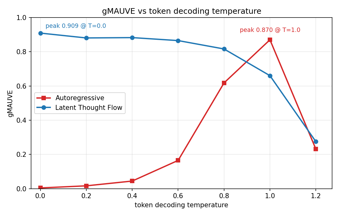
Decoder-temperature sweep at fixed readout model size. Token AR (red) needs non-greedy sampling to reach its ceiling, while Latent Thought Flows (blue) remain strong near greedy decoding.
Two things stand out:
- Greedy already works for LTF. At T=0.0, where the decoder is fully deterministic given the latent, LTF still reaches gMAUVE 0.909. Under this evaluation, decoder-side greedy AR collapses to low distributional diversity, while LTF still varies because each sample draws a different latent plan from noise. The LTF readout does not need decoder-side randomness to produce a varied, distribution-matching corpus.
- The LTF peak sits at very low temperature. The plotted peak is at T=0.0, and the curve stays near its maximum over a low-temperature plateau before degrading as temperature rises.
Together these say that in LTF the readout decoder is doing very little sampling work. Almost all of the per-sample variability that MAUVE measures has already been injected upstream — by the MeanFlow generator drawing a fresh latent sequence from Gaussian noise. The decoder's job is to faithfully read out that latent into surface text, which is best done at low or zero temperature. In the AR baseline, by contrast, the decoder has no upstream entropy source, so distributional diversity has to come from token-by-token sampling, which is why it needs a non-greedy temperature in this evaluation and why it is temperature-fragile.
This is the structural reason the gap in the previous figures is persistent: it is not that LTF is a better-tuned sampler on top of the same base model. It is that LTF moves the entropy out of the readout step and into a continuous latent generator, where it can be modeled directly.
We now ask two questions. First, does the latent space have usable geometry for generation? Second, does an individual latent code causally control the samples produced by the readout? We address the geometry question first, then return to direct latent-control probes.
Evaluating Latent Quality
Everything above rests on one assumption: that the flow model has a good latent space to learn on. So what makes a latent space good? The obvious answer — that the autoencoder reconstructs its input faithfully — turns out to be the wrong one.
The core question is not whether the autoencoder can reconstruct, but whether its latent space is shaped for generation. Reconstruction metrics answer the first question; they say nothing about the second. The short version is: reconstruction is not enough; interpolation predicts generation.
MAUVE [7] gives a distributional comparison for text: it embeds generated and reference text with a pretrained language model and compares the two resulting distributions. We use it in three ways. rMAUVE measures decoded reconstructions, gMAUVE measures samples from a learned latent generator, and iMAUVE measures interpolations in the learned latent space.
For iMAUVE, we retrieve a nearest neighbor for each real text example in latent space, decode the midpoint between the two latent codes, and compare these decoded midpoints to held-out text. A good iMAUVE score means that local interpolation paths stay on the text manifold, which is exactly the structure a downstream flow model needs.
Why interpolation, and why the nearest-neighbor midpoint?
This distinction has a direct precedent in image generation. The iFID paper [6] showed that reconstruction FID is poorly correlated with the generation FID of a latent diffusion model trained on top of the VAE. The metric that does predict generation quality is interpolated FID: for each real image, retrieve its nearest neighbor in latent space, decode the midpoint of the two latents, and compute FID against real data. The nearest-neighbor step is the key: it probes interpolation between nearby points on the latent manifold, which is the regime a diffusion sampler actually traverses.
Our iMAUVE protocol is the text analogue. It is not trying to reward exact reconstruction. It asks whether the learned latent geometry is locally filled in by plausible text.
In this sweep, rMAUVE is effectively uninformative: reconstructions stay near-perfect even as generation quality changes substantially. iMAUVE is the useful signal here. Across the tested autoencoder configurations, iMAUVE tracks gMAUVE closely (Pearson r = +0.95), while rMAUVE stays saturated and does not separate good latent spaces from bad ones (r = -0.62).
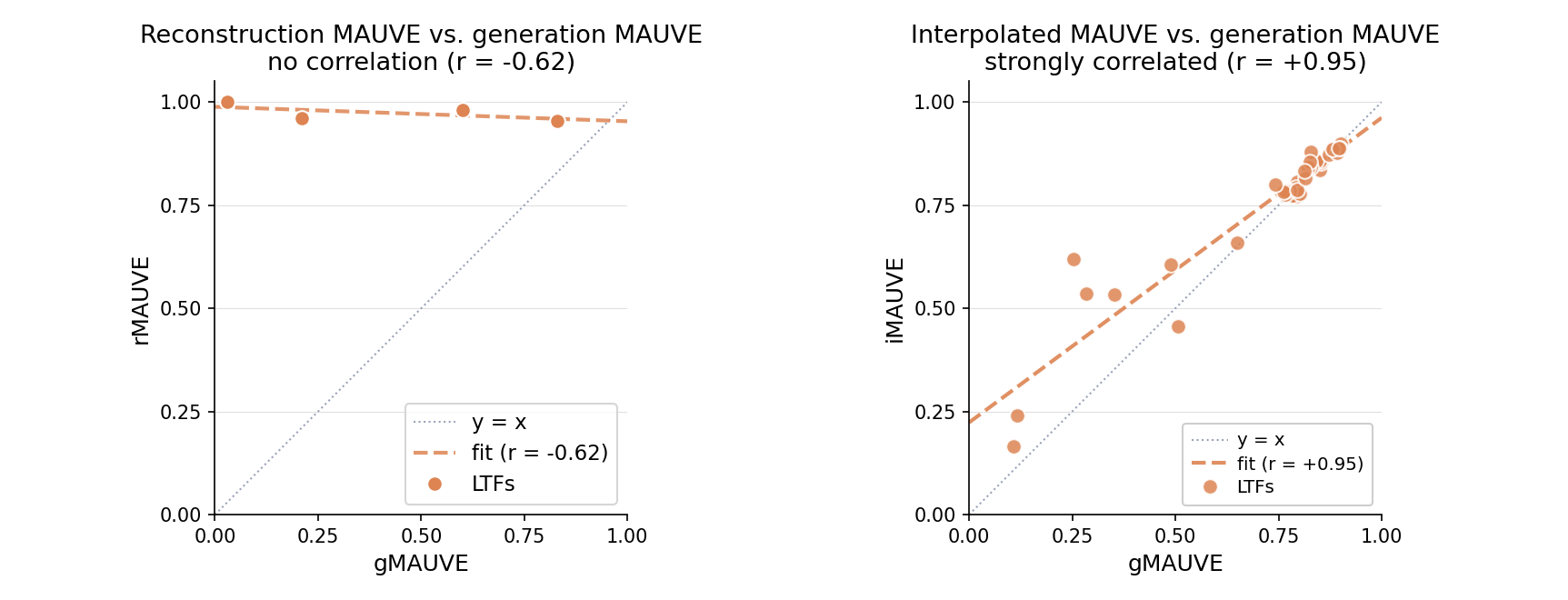
Left: rMAUVE saturates near 1.0 and fails to distinguish useful from unusable latents. Right: iMAUVE tracks downstream generation quality in this sweep.
The qualitative takeaway is simple: good latents change decoded text smoothly. Moving along a latent direction changes story attributes without collapsing, and interpolating between nearby latents produces fluent midpoint stories. These demos are not additional metrics; they make the geometry visible.
Good vs. bad latent evidence
To make the rMAUVE / iMAUVE distinction concrete, we visualize the latent spaces of two autoencoders on the same 2000-story TinyStories validation set. Both reconstruct the input text well. Only one has a latent space whose midpoints decode into coherent stories.
| Good latent | Bad latent | |
|---|---|---|
| rMAUVE (reconstruction → real text) | ≈ 0.95 (paraphrase-quality) | 1.00 (near-verbatim) |
| iMAUVE (midpoint → real text) | 0.78 | 0.005 |
| Reconstruction style | Same characters and arc, reworded surface | Source story copied with sporadic token swaps |
| Interpolation style | Coherent blend of two real stories | Fluent prefix then token soup |
Reading rMAUVE alone, the bad latent looks like the better autoencoder — its reconstructions are nearly verbatim. iMAUVE drops by more than two orders of magnitude across the same axis. The latent space is decodable at real encodings but not between them.
Same anchor, two latent spaces
Take a fixed anchor story, retrieve its nearest neighbor in each latent space, and decode (a) the anchor's own latent and (b) the midpoint between the anchor and that neighbor:
Anchor (real story): "Once upon a time, there was a big dog named Max. Max had a red collar that he wore every day. He loved to play and run in the park with his friends. One day, Max saw a cat on a tree…"
| Good latent (iMAUVE = 0.78) | Bad latent (iMAUVE = 0.005) | |
|---|---|---|
| Reconstruction (decode anchor's own latent) | "Once upon a time, there was a big dog named Max. Max had a long tail that he loved to play with. He would run and jump all day long. One day, Max saw a cat in the park. The cat had a big red bow on its head…" | "Once upon a time, there was a big dog named Max. Max had a red collar that he walking every day. He loved to play and run in the park with his friends. One day, Max saw a cat on a tree. He wanted to be friends with the cat. So, Max tried t[o]…" |
| Midpoint (decode α=0.5 between anchor and nearest-neighbor latent) | "Once upon a time, there was a little dog named Max. Max loved to play in the park. He had a big ball with him. He would run and jump all day long. One day, Max saw a big red ball in the park. He wanted to play with the ball, but he couldn't…" | "Once upon a time, there was a little boy named Max. She had a a jacket that he loved to explore. One went, Tim he not in the park and his much. But, Max saw a and on one. You do that you friends friend his replied…" |
The good latent paraphrases the anchor — same characters, same arc, reworded surface — and produces a fluent blended story at the midpoint between two real encodings. The bad latent copies the anchor at the token level and then disintegrates into token soup at the midpoint, even though both endpoints of that interpolation are themselves encodings of real, fluent stories.
Nearest neighbors: semantics vs. length
The midpoint test asks what lies between two encodings. A complementary test asks what lies near an encoding: for a given anchor story, what does each latent space consider its closest neighbors?
The pattern is consistent across anchors. In the good space, neighbors share characters, register, or narrative shape. In the bad space, neighbors share mostly word count — the bad latent's principal axis correlates with story length at r = 0.93, and nearest neighbors differ from the anchor by an average of just 10 words.
Anchor: "A kind doctor helped a little girl with a boo-boo on her knee." (134 words)
| Good latent — emotional-tone cluster (sadness, insufficiency) | Bad latent — ~134-word stories, unrelated content |
|---|---|
| Dull the horse. He was not very happy because… | A girl who was very worried. She wanted to make herself look pretty… |
| A bald man named Tom. Tom loved to print pictures but was very miserable… | Ducky the duck loved to play in the pond with his friends… |
| A little train named Toot. Toot was very miserable. He did not like to work… | A poor neighbor who had a big cat. The cat was very fat and heavy… |
| An elderly boat named Bob. Bob lived in a big port… | A big hairy rabbit named Bongo who loved to eat radishes… |
The good space surfaces Dull, miserable, miserable, elderly — a pure emotional-register cluster around sadness and insufficiency, which fits the doctor story's "someone coming to fix hurt things" shape. The bad space instead retrieves unrelated stories with nearly the same length.
Additional nearest-neighbor examples
Anchor: "Once upon a time, there was a tiny spider called Jasper. He spun a beautiful cobweb every day." (158 words)
| Good latent — small beings striving in their role | Bad latent — ~158-word stories |
|---|---|
| A stubborn seed that wanted to bloom like all the other flowers… | Peter was excited to play with water in the backyard… |
| A hairy pup so small it could fit in one hand… | A caterpillar who wanted to measure flowers and trees… |
| An enormous bubble that was not happy. It wanted to impress everyone… | A girl named Anne who had a very special wish… |
| A famous factory called 'Happy Factory' that made lots of toys… | Two friends who really loved hockey… |
Jasper, the seed, the tiny pup, the bubble — all small things striving to do the thing they're meant to do. The good space organizes by narrative shape, not surface noun.
Anchor: "Once upon a time there was a big dragon. Fire would come out of its mouth." (173 words)
| Good latent — mythic-scale creatures and places | Bad latent — ~173-word stories |
|---|---|
| A compassionate owl beloved by all the woodland creatures… | A furry bear who kept the forest safe… (also retrieved by the good latent — a length coincidence) |
| A furry bear, very brave, who kept the forest safe… | A curious little fox who explored the forest every day… |
| An ancient castle, very big, with high walls… | A big tough bear who liked walks in the woods… |
| A big tough bear who liked walks in the woods… | A brave fish in the deep blue sea… |
The two spaces happen to share one neighbor (the bear), but only because long stories skew toward forest/fantasy — the bad space's other neighbors (curious fox, brave fish) lack the dragon's mythic scale entirely.
Across anchors, the good latent's neighbors are bound by what the story is about; the bad latent's are bound by how long it is. This is what the iMAUVE gap is measuring at the scale of individual points.
This is the iMAUVE failure mode in microcosm. A latent space that reconstructs perfectly can still collapse off the data manifold the moment you step between two real points — exactly the regime a downstream continuous generator has to operate in. Once you have iMAUVE as a metric, an rMAUVE-only selection criterion becomes actively misleading: it would tell you the bad latent is the better autoencoder.
Probing What the Latent Controls
The metrics above test whether the latent space has useful geometry. A separate question is causal: what does a single latent code actually control when the readout decoder samples text?
The answer we want is not memorization. A good latent should not be a lookup key for one exact sequence. It should fix the semantic plan of the text — character, setting, goal, rough event structure — while leaving the readout decoder free to realize that plan in different surface forms.
Fixed-Latent Sampling
We fix one latent code and sample the readout decoder many times, changing only the readout sampling noise. If the readout ignores the latent, these samples should behave like an unconditional TinyStories language model. If the latent is doing real work, the samples should share story-level content while varying in phrasing.
Fixed-latent sampling demo
Qualitatively, repeated samples from the same latent share the same story skeleton: the main character, setting, goal, and rough event structure are stable. What changes is the surface realization: wording, names, minor objects, and local transitions. This is the behavior we want from a text latent. The latent controls the semantic plan; the readout decoder realizes that plan stochastically in text.
Latent Intervention Probes
We also test the reverse direction: if we replace the latent, does the generated story move with it?
It does. Matched real latents preserve source-level content. Shuffled real latents transfer generated samples toward the donor latent rather than the original source. Invalid latents such as zero, mean, or noise collapse both anchoring and distributional quality.
This rules out the simplest failure mode: the readout is not merely an unconditional language model with a decorative latent prefix. Its samples depend causally on the latent sequence.
Intervention details
The intervention test keeps the target text fixed, then replaces the latent sequence by matched, shuffled, zero, mean, or noise latents. For 10M-25M readout decoders, shuffling latents increases CE by roughly 4.0-4.3, while zero/mean/noise interventions still increase CE by roughly 2.6-3.3. The degradation is already visible in the first 64 token positions, where local teacher-forced context gives the readout the best chance to recover.
The same conclusion appears in free-sampling retrieval probes. For each generated sample, we retrieve the nearest source text under an external text embedding model. Source top-1 means the generated text retrieves its own source; donor top-1 means it retrieves the source whose latent was inserted after shuffling. Duplicate rate is the fraction of repeated generations among 16 samples from the same source.
| intervention | prediction if z is ignored | observed | conclusion |
|---|---|---|---|
| matched real z, 16 samples/source | source retrieval near random | source top-1 0.85-0.89; duplicate rate 0 | z preserves source-level content without becoming a lookup table |
| shuffled real z | swapping z should not systematically move the story | donor top-1 0.85-0.90; original-source top-1 near 0 | generated content follows the donor latent, not the original index |
| zero z | zero z should behave like real z | source top-1 0.01-0.02; marginal MAUVE drops to 0.01-0.09 | off-manifold latents lose both anchoring and distributional quality |
Shuffled latents still come from the real encoder marginal, so their unpaired text distribution can look good. The paired retrieval probe resolves the ambiguity: those samples follow the donor latent rather than the original source.
What Makes the Latents Useful for Generation?
The autoencoder should be trained as a representation learner, not merely as a reconstruction machine. The central pattern is that good text latents require pressure from both sides: the encoder must summarize rather than route surface form, and the readout decoder must read from the latent rather than behave like an ordinary language model.
Concretely, three mechanisms mattered most in our experiments. First, force the encoder to summarize instead of copying visible tokens through the bottleneck. Second, make the readout depend on the latent instead of recovering the sequence as an ordinary language model. Third, give the readout enough local text context to write fluent text, but not so much context that it becomes a full bypass around the latent.
i. Force Summarization Instead of Routing
The first pressure is on the encoder. During encoder training, we randomly keep only a subset of the input tokens, preserve their positions, and ask the latent queries to reconstruct the full sequence. This is MAE-style dropping [3], but applied to text compression and closely related to denoising sequence-to-sequence objectives in BART, T5, and MASS [9, 10, 11].
The effect is simple: the encoder cannot solve the task by copying most of the surface form. It must infer missing context and summarize it into the latent tokens. This changes the statistical task and also reduces encoder compute, since the bidirectional encoder sees fewer tokens.
Empirically, too little dropping leaves the encoder free to route visible tokens; with more training, this easy reconstruction route does not produce a stable interpolation geometry. Stronger dropping makes the encoder infer missing context and summarize it into the latent slots. This is why MAE drop is not just a compute trick: it changes the optimization path toward latents that remain meaningful under interpolation.
ii. Make the Readout Depend on the Latent
The second pressure is on the readout. Because the readout decoder is autoregressive in our implementation and highly expressive, it can learn to rely mostly on previous-token context and underuse the encoded latents. This is analogous to posterior collapse in language VAEs [8, 12], where a strong decoder can model the sequence while ignoring the latent variable. When this happens, the training signal largely bypasses the encoder, so the learned codes may reconstruct locally but fail to become useful generative latents.
We therefore randomly drop the readout decoder's access to previous-token context during training, with probability p_{\mathrm{dec}}. When previous tokens are masked, the latent prefix becomes the main source of information, which encourages the readout to condition on the encoder output.
The probing section above gives the corresponding evidence: fixed-latent sampling preserves story-level content, shuffled latents transfer donor semantics, and invalid latents collapse generation. The readout can exploit local context, but the latent slots still carry essential example-specific information.
iii. Give the Readout Local Context, But Not a Full Bypass
The third pressure is a balance. The readout needs enough local text context to write fluent sequences, but too much context can become a bypass around the latent. We control this with sliding-window attention: each position can attend to the latent prefix and only a limited window of previous text tokens.
This also gives a useful diagnostic. We compare two regimes while sweeping the decoder's sliding-window size:
- Latent Thought Flows: the full Stage-1 recipe, where encoder and decoder are trained jointly and the latent tokens are per-example.
- Constant-prefix AR baseline: the encoder is bypassed and the decoder is trained with learned constant prefix vectors. Per-example latent content is removed, so any remaining gMAUVE is what a strong autoregressive decoder with a soft prompt can achieve on its own.
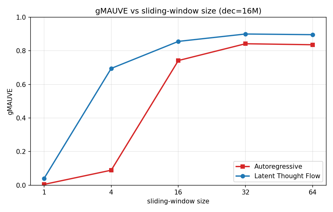
Sliding-window sweep at decoder = 16M. Latent Thought Flows stay above the constant-prefix AR baseline across window sizes.
Two lessons follow. First, the sliding window is not a minor implementation detail: without a useful text window, both curves collapse; with an appropriate window, the readout has enough local context to write fluent text while still needing the latent prefix. Second, a stronger decoder is not a substitute for a meaningful per-example latent — the constant-prefix AR baseline can recover part of the distributional prior, but Latent Thought Flows still win at matched window size.
Bottleneck parameterization and latent bandwidth
Two additional sweeps help bound the recipe.
Bottleneck parameterization
The main recipe in this post uses a deterministic continuous bottleneck trained with autoregressive reconstruction. We also tested VAE-style stochastic bottlenecks, related to language latent-space models such as Optimus [5], with a KL penalty. In this from-scratch recipe, they optimized reconstruction but did not produce useful interpolation geometry.
This should be interpreted as a limitation of this specific setup, not as a claim that language VAEs are ineffective. Pretrained representations, masked or parallel readouts, diffusion/flow decoders, or stronger anti-collapse objectives could make stochastic bottlenecks viable.
For scale, in our TinyStories sweep, with patch size 256 and 32x token compression (K = 8 latent tokens), the best AR autoencoder reaches iMAUVE 0.891, while the best VAE-style run remains near zero:
| objective | KL weight | iMAUVE |
|---|---|---|
| deterministic AE | - | 0.891 |
| best VAE-style bottleneck | 0.001 | 0.0056 |
The other KL weights we tested are in the same range, about 0.004-0.006 iMAUVE.
Latent bandwidth
There are two natural bandwidth axes: the number of latent tokens K and the channel dimension d. They jointly determine the rough latent bandwidth Kd, but they play different computational roles: K controls how many continuous slots represent a text span, while d controls the per-slot information channel.
Compression helps shape the latent space. In our sweeps, moderate-to-heavy token compression remains strong over a wide range, suggesting that a real bottleneck can improve the latent geometry. Increasing the channel dimension d improves iMAUVE until it plateaus, so the useful capacity seems to come from enough per-latent bandwidth together with pressure to summarize across tokens.
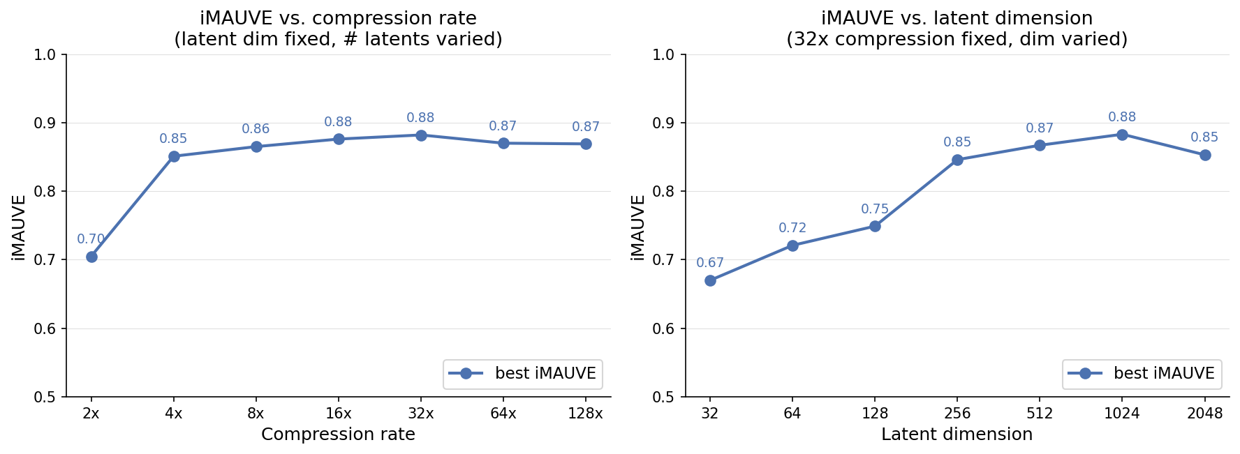
Compression and channel-dimension sweeps on TinyStories (patch=256). Moderate-to-heavy token compression remains strong over a wide range, while increasing d improves iMAUVE until it plateaus.
Beyond representation quality, compression has a direct effect on generation cost: fewer latent tokens means a shorter sequence and a cheaper pass for the flow model, before the readout decoder expands them back to text.
Method Details
The method has two stages. First, train a text autoencoder that maps a token sequence into a short sequence of continuous latent tokens. Second, freeze that autoencoder and train a latent MeanFlow model to generate those latent tokens from noise. The readout decoder then maps the generated latents back into text.
Stage 1: Text Autoencoder
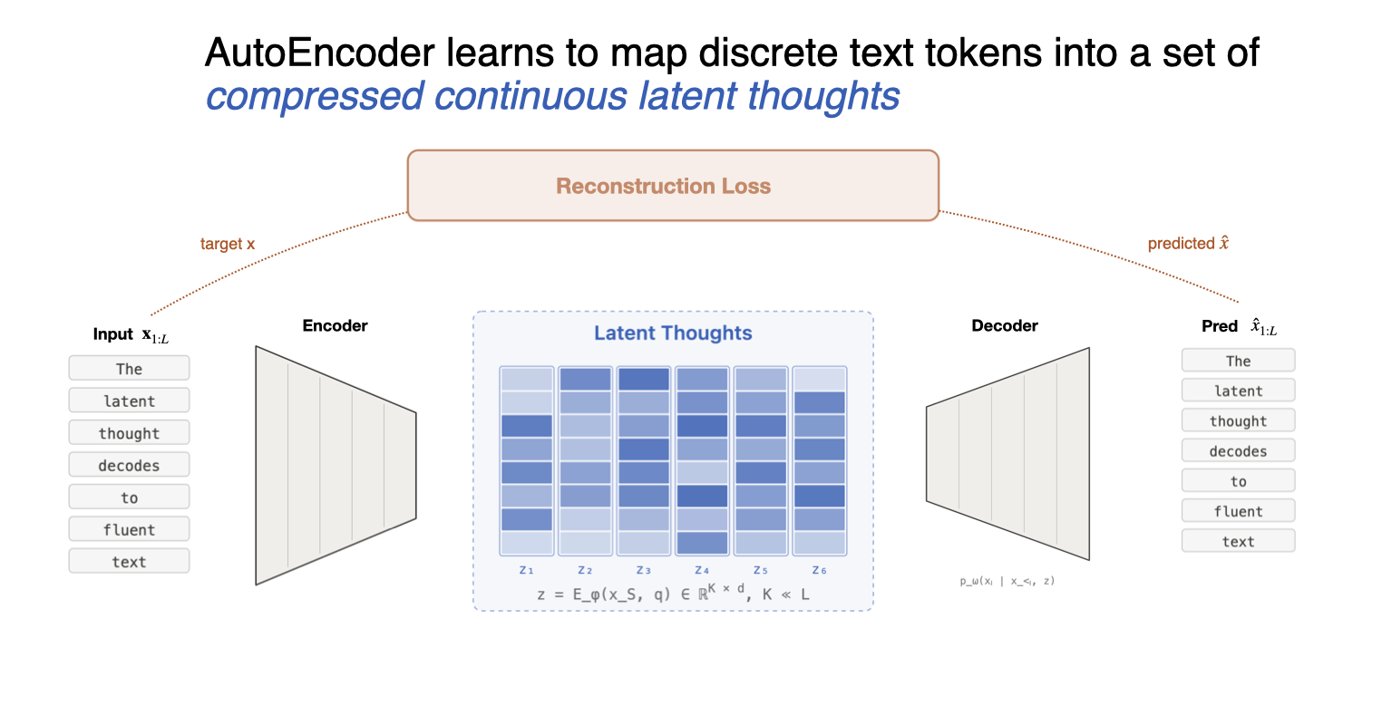
Stage 1 training. The encoder compresses a text patch into K continuous latent tokens, and the readout decoder reconstructs the full sequence from that latent prefix. These latent slots are what the Stage 2 generator later models.
Let a text patch contain L token ids. The encoder maps it into K continuous latent tokens, with K \ll L. The readout decoder is conditioned on those latents and reconstructs the full sequence. In our current implementation, the readout is a causal language model conditioned on a latent prefix or memory.
This separates representation learning from text readout. The encoder can be bidirectional and summarize the whole patch, while the readout decoder maps the latent sequence back to text. In practice, the key training choice is to make the encoder view sparse enough that the latent tokens must summarize missing context rather than route surface tokens.
Autoencoder objective and implementation notes
Let a text patch be a sequence of token ids
The main risk is that a powerful encoder can route surface tokens through the bottleneck without learning useful global structure. We therefore train the encoder with a sparse input view: during encoder training, we randomly keep only a visible subset of input tokens, preserve their positions, and ask the latent queries to reconstruct the full sequence.
The encoder maps the sequence into continuous latent tokens:
The readout decoder models
For the current autoregressive readout,
During sparse encoder training, we keep a visible subset
The encoder sees only the visible tokens with their original positions, plus learned latent queries:
Stochastic VAE-style variants are discussed in the bottleneck section above; the main recipe here uses deterministic latent tokens.
MAE-style dropping also shortens the bidirectional encoder sequence. If the full encoder length is n_0=L+K and the dropped length is n_1=|S|+K, a per-layer Transformer block proxy is
The attention term decreases quadratically with sequence length, while projections and MLP terms decrease linearly. The more important effect is statistical: dropping changes the task so the latent sequence must predict missing content.
Stage 2: Latent MeanFlow Generator
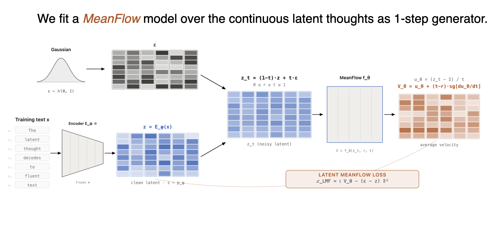
Stage 2 training. With the autoencoder frozen, real latents from the Stage 1 encoder are mixed with Gaussian noise. A MeanFlow network learns the average velocity needed to jump from noisy latents back to clean latents, after which the readout decoder expands them into text.
Compression makes the generative problem cheaper only if the latent generator is cheap. Instead of generating L text tokens directly, the latent model generates only K continuous tokens; MeanFlow targets the one-step regime where latent generation is a small overhead and the readout decoder remains the dominant cost.
MeanFlow is useful here because it is designed for fast motion from Gaussian noise to a structured data manifold. After text compression, the encoder-induced latents form exactly such a manifold: most ambient points in \mathbb{R}^{K\times d} are not valid text latents. Stage 2 models this short continuous manifold rather than solving token-by-token language modeling directly.
The trajectory demos make this object visible: the flow model moves through a short continuous text-latent space, and the readout decoder turns that path into text.
MeanFlow sampling trajectory
Latent geometry trajectory
At training time, we encode real text into clean latents, mix those latents with Gaussian noise, and train a MeanFlow network to map noisy latents back toward the encoder manifold. At inference, sampling starts from Gaussian noise in latent space and decodes the resulting latent tokens into text.
MF in High-dimensional Latent Space
Let the latent distribution induced by the encoder be p_\phi(\mathbf{z}). Sample a clean latent and Gaussian noise:
Define the linear path from data to noise:
This is a high-dimensional ambient-space problem with low-dimensional data structure: valid text latents occupy the encoder-induced manifold inside \mathbb{R}^{K\times d}, while Gaussian noise fills the ambient space. Following the data-prediction MeanFlow formulations in Pixel Mean Flows and Improved Mean Flows [4, 21], the network predicts the clean latent sequence,
This data prediction induces an average-velocity prediction:
The MeanFlow identity then turns this into a compound instantaneous-velocity prediction:
where the total derivative is taken along the path
The MF loss matches this compound prediction to the true path velocity:
Here sg denotes stop-gradient. This keeps the training target stable while still using the model's tangent information to construct the interval velocity.
Related aside: how about direct text diffusion?
A natural comparison is to diffuse or flow directly over text tokens, token embeddings, or learned text latents. Several lines of work are close to this question.
Language VAEs and learned text latents. Sentence VAEs and Optimus study continuous sentence-level latent variables for language generation [12, 5], and neural text compression studies learned compressed representations for language modeling [2]. These works make clear why reconstruction alone is not enough: strong decoders can underuse the latent, and good reconstruction does not guarantee a latent space that is easy to generate from.
Latent diffusion over learned text latents. LD4LG compresses text with a language autoencoder, runs diffusion in the autoencoder latent space, and decodes the sampled latents back to language [26]. PLANNER combines latent semantic diffusion with autoregressive decoding to generate paragraph-level plans [27]. Latent Thought Flows are in the same broad family, but shift the focus from diffusion to the representation: the learned text latents must be short, reconstructive, interpolable, and generative, so that a one-step latent generator can model them directly.
Discrete diffusion over token states. One route keeps the state space discrete. Early categorical diffusion work includes Multinomial Diffusion and D3PM-uniform, where the corruption process can transition toward a uniform categorical state [33, 34]. Later discrete language diffusion methods use objectives closer to token modeling: score-entropy ratio estimation in SEDD [18], and masked-token diffusion, scaled first to billion-parameter models with a scaling law comparable to autoregressive training [19], and then to LLaDA, an 8B diffusion language model trained from scratch that competes with autoregressive LLMs of the same size [37]. Recent systems such as DiffusionGemma scale this uniform-state discrete diffusion direction to larger text models [35].
Continuous diffusion or flow over token embeddings. A second route keeps the sequence length L but moves each token into a continuous embedding space. Diffusion-LM and likelihood-based diffusion language models denoise full sequences of continuous word or token embeddings and then round back to text [16, 17]. CDCD keeps diffusion continuous in time and input space while modeling categorical data such as language [29]. LangFlow connects embedding-space diffusion language modeling to Flow Matching through a Bregman-divergence view and trains with a cross-entropy objective [28]. ELF formulates language generation as continuous-time Flow Matching in embedding space and discretizes only at the final step [31].
Hybrid and joint-state models. A third group hybridizes along one of two axes: the generation order, or the state space itself. On the order axis, SSD-LM generates blocks of text semi-autoregressively while diffusing within each block [36], and Block Diffusion makes that split explicit, running autoregressive generation across blocks and diffusion-style generation inside them [20]. On the state axis, SSD-LM already relaxes the discrete vocabulary into a simplex rather than a learned embedding space, and two concurrent systems carry both states at once: CADD pairs the discrete chain with a diffusion in continuous latent space, so a masked token becomes a noisy but informative latent rather than an information void [38], while CCDD treats the continuous representation state and the discrete token state as co-equal and denoises both jointly [32].
Continuous thought. Coconut explores reasoning in continuous hidden-state space rather than always decoding intermediate thoughts into words [30]. That motivation is related, but the task here is different: we are testing whether compressed continuous latents can serve as a generative interface for text itself.
The central distinction is therefore not "diffusion versus autoregression." It is where the continuous generative model operates. Token- and embedding-space flow/diffusion models denoise length-L text states. Latent Thought Flows first compress text into K continuous latent tokens, with K \ll L, and model that shorter latent sequence before the readout decoder turns it back into text.
What This Suggests
The main lesson is that text latents should be judged as generative objects, not reconstruction codes. Sparse encoder bottlenecks and generation-aware evaluations make this distinction visible. The evidence here says that text can live in a compact continuous latent space that supports generation, not merely reconstruction.
The next questions are scale, general-domain text, and reasoning. Can the same interface work beyond TinyStories, with larger corpora, longer contexts, and tasks where the latent must carry abstract plans rather than short narrative structure?
For autoregressive modeling, the message is not to discard token readout, but to condition it on a generated latent plan. For flow and diffusion modeling, the message is not to denoise raw text tokens, but to model a compact continuous state that text can be read from. Latent Thought Flows are an attempt to make these two views meet.
References
[1] Grégoire Delétang, Anian Ruoss, Paul-Ambroise Duquenne, Elliot Catt, Tim Genewein, Christopher Mattern, Jordi Grau-Moya, Li Kevin Wenliang, Matthew Aitchison, Laurent Orseau, Marcus Hutter, and Joel Veness. Language Modeling Is Compression. ICLR 2024.
[2] Brian Lester, Jaehoon Lee, Alexander A. Alemi, Jeffrey Pennington, Adam Roberts, Jascha Sohl-Dickstein, and Noah Constant. Training LLMs over Neurally Compressed Text. Transactions on Machine Learning Research, 2024.
[3] Kaiming He, Xinlei Chen, Saining Xie, Yanghao Li, Piotr Dollár, and Ross Girshick. Masked Autoencoders Are Scalable Vision Learners. CVPR 2022.
[4] Yiyang Lu, Susie Lu, Qiao Sun, Hanhong Zhao, Zhicheng Jiang, Xianbang Wang, Tianhong Li, Zhengyang Geng, and Kaiming He. One-step Latent-free Image Generation with Pixel Mean Flows. arXiv:2601.22158, 2026.
[5] Chunyuan Li, Xiang Gao, Yuan Li, Baolin Peng, Xiujun Li, Yizhe Zhang, and Jianfeng Gao. Optimus: Organizing Sentences via Pre-trained Modeling of a Latent Space. EMNLP 2020.
[6] Tongda Xu, Mingwei He, Shady Abu-Hussein, José Miguel Hernández-Lobato, Haotian Zhang, Kai Zhao, Chao Zhou, Ya-Qin Zhang, and Yan Wang. Making Reconstruction FID Predictive of Diffusion Generation FID. arXiv:2603.05630, 2026.
[7] Krishna Pillutla, Swabha Swayamdipta, Rowan Zellers, John Thickstun, Sean Welleck, Yejin Choi, and Zaid Harchaoui. MAUVE: Measuring the Gap Between Neural Text and Human Text using Divergence Frontiers. NeurIPS 2021.
[8] Junxian He, Daniel Spokoyny, Graham Neubig, and Taylor Berg-Kirkpatrick. Lagging Inference Networks and Posterior Collapse in Variational Autoencoders. ICLR 2019.
[9] Mike Lewis, Yinhan Liu, Naman Goyal, Marjan Ghazvininejad, Abdelrahman Mohamed, Omer Levy, Veselin Stoyanov, and Luke Zettlemoyer. BART: Denoising Sequence-to-Sequence Pre-training for Natural Language Generation, Translation, and Comprehension. ACL 2020.
[10] Colin Raffel, Noam Shazeer, Adam Roberts, Katherine Lee, Sharan Narang, Michael Matena, Yanqi Zhou, Wei Li, and Peter J. Liu. Exploring the Limits of Transfer Learning with a Unified Text-to-Text Transformer. Journal of Machine Learning Research, 21(140):1-67, 2020.
[11] Kaitao Song, Xu Tan, Tao Qin, Jianfeng Lu, and Tie-Yan Liu. MASS: Masked Sequence to Sequence Pre-training for Language Generation. ICML 2019.
[12] Samuel R. Bowman, Luke Vilnis, Oriol Vinyals, Andrew M. Dai, Rafal Jozefowicz, and Samy Bengio. Generating Sentences from a Continuous Space. CoNLL 2016.
[13] Robin Rombach, Andreas Blattmann, Dominik Lorenz, Patrick Esser, and Björn Ommer. High-Resolution Image Synthesis with Latent Diffusion Models. CVPR 2022.
[14] Jesse Mu, Xiang Lisa Li, and Noah Goodman. Learning to Compress Prompts with Gist Tokens. NeurIPS 2023.
[15] Alexis Chevalier, Alexander Wettig, Anirudh Ajith, and Danqi Chen. Adapting Language Models to Compress Contexts. EMNLP 2023.
[16] Xiang Lisa Li, John Thickstun, Ishaan Gulrajani, Percy Liang, and Tatsunori B. Hashimoto. Diffusion-LM Improves Controllable Text Generation. NeurIPS 2022.
[17] Ishaan Gulrajani and Tatsunori B. Hashimoto. Likelihood-Based Diffusion Language Models. NeurIPS 2023.
[18] Aaron Lou, Chenlin Meng, and Stefano Ermon. Discrete Diffusion Modeling by Estimating the Ratios of the Data Distribution. ICML 2024.
[19] Shen Nie, Fengqi Zhu, Chao Du, Tianyu Pang, Qian Liu, Guangtao Zeng, Min Lin, and Chongxuan Li. Scaling up Masked Diffusion Models on Text. ICLR 2025.
[20] Marianne Arriola, Aaron Gokaslan, Justin Chiu, Zhihan Yang, Zhixuan Qi, Jiaqi Han, Subham Sahoo, and Volodymyr Kuleshov. Block Diffusion: Interpolating Between Autoregressive and Diffusion Language Models. ICLR 2025.
[21] Zhengyang Geng, Yiyang Lu, Zongze Wu, Eli Shechtman, J. Zico Kolter, and Kaiming He. Improved Mean Flows: On the Challenges of Fastforward Generative Models. CVPR 2026.
[22] Jared Kaplan, Sam McCandlish, Tom Henighan, Tom B. Brown, Benjamin Chess, Rewon Child, Scott Gray, Alec Radford, Jeffrey Wu, and Dario Amodei. Scaling Laws for Neural Language Models. arXiv:2001.08361, 2020.
[23] Jordan Hoffmann, Sebastian Borgeaud, Arthur Mensch, Elena Buchatskaya, Trevor Cai, Eliza Rutherford, Diego de Las Casas, Lisa Anne Hendricks, Johannes Welbl, Aidan Clark, Tom Hennigan, Eric Noland, Katie Millican, George van den Driessche, Bogdan Damoc, Aurelia Guy, Simon Osindero, Karen Simonyan, Erich Elsen, Jack W. Rae, Oriol Vinyals, and Laurent Sifre. Training Compute-Optimal Large Language Models. arXiv:2203.15556, 2022.
[24] Zhengyang Geng, Mingyang Deng, Xingjian Bai, J. Zico Kolter, and Kaiming He. Mean Flows for One-step Generative Modeling. NeurIPS 2025.
[25] Ronen Eldan and Yuanzhi Li. TinyStories: How Small Can Language Models Be and Still Speak Coherent English?. arXiv:2305.07759, 2023.
[26] Justin Lovelace, Varsha Kishore, Chao Wan, Eliot Shekhtman, and Kilian Q. Weinberger. Latent Diffusion for Language Generation. NeurIPS 2023.
[27] Yizhe Zhang, Jiatao Gu, Zhuofeng Wu, Shuangfei Zhai, Joshua Susskind, and Navdeep Jaitly. PLANNER: Generating Diversified Paragraph via Latent Language Diffusion Model. NeurIPS 2023.
[28] Yuxin Chen, Chumeng Liang, Hangke Sui, Ruihan Guo, Chaoran Cheng, Jiaxuan You, and Ge Liu. LangFlow: Continuous Diffusion Rivals Discrete in Language Modeling. arXiv:2604.11748, 2026.
[29] Sander Dieleman, Laurent Sartran, Arman Roshannai, Nikolay Savinov, Yaroslav Ganin, Pierre H. Richemond, Arnaud Doucet, Robin Strudel, Chris Dyer, Conor Durkan, Curtis Hawthorne, Rémi Leblond, Will Grathwohl, and Jonas Adler. Continuous Diffusion for Categorical Data. arXiv:2211.15089, 2022.
[30] Shibo Hao, Sainbayar Sukhbaatar, DiJia Su, Xian Li, Zhiting Hu, Jason Weston, and Yuandong Tian. Training Large Language Models to Reason in a Continuous Latent Space. COLM 2025.
[31] Keya Hu, Linlu Qiu, Yiyang Lu, Hanhong Zhao, Tianhong Li, Yoon Kim, Jacob Andreas, and Kaiming He. ELF: Embedded Language Flows. arXiv:2605.10938, 2026.
[32] Cai Zhou, Chenxiao Yang, Yi Hu, Chenyu Wang, Chubin Zhang, Muhan Zhang, Lester Mackey, Tommi Jaakkola, Stephen Bates, and Dinghuai Zhang. Coevolutionary Continuous Discrete Diffusion: Make Your Diffusion Language Model a Latent Reasoner. ICML 2026.
[33] Emiel Hoogeboom, Didrik Nielsen, Priyank Jaini, Patrick Forré, and Max Welling. Argmax Flows and Multinomial Diffusion: Learning Categorical Distributions. NeurIPS 2021.
[34] Jacob Austin, Daniel D. Johnson, Jonathan Ho, Daniel Tarlow, and Rianne van den Berg. Structured Denoising Diffusion Models in Discrete State-Spaces. NeurIPS 2021.
[35] Google. Introducing DiffusionGemma. Google Blog, 2026.
[36] Xiaochuang Han, Sachin Kumar, and Yulia Tsvetkov. SSD-LM: Semi-autoregressive Simplex-based Diffusion Language Model for Text Generation and Modular Control. ACL 2023.
[37] Shen Nie, Fengqi Zhu, Zebin You, Xiaolu Zhang, Jingyang Ou, Jun Hu, Jun Zhou, Yankai Lin, Ji-Rong Wen, and Chongxuan Li. Large Language Diffusion Models. arXiv:2502.09992, 2025.
[38] Huangjie Zheng, Shansan Gong, Ruixiang Zhang, Tianrong Chen, Jiatao Gu, Mingyuan Zhou, Navdeep Jaitly, and Yizhe Zhang. Continuously Augmented Discrete Diffusion model for Categorical Generative Modeling. ICLR 2026.
How to cite
Mihir Prabhudesai and Zhengyang Geng. “Latent Thought Flows with Text Compression.” 2026.
@techreport{ltf2026latent,
  title       = {Latent Thought Flows with Text Compression},
  author      = {Prabhudesai, Mihir and Geng, Zhengyang},
  institution = {Carnegie Mellon University},
  year        = {2026},
  url         = {https://latent-thought-flows.vercel.app/}
}